A number of circles are being completed by this year’s workshop at the University of Ljubljana on Risk and Artificial Intelligence.

• The previous workshop was my last talk for non-virtual people before Covid lockdowns, and this workshop is my first post-lockdown
• The EU’s proposed AI Act and the German regulator’s IT Requirements for Asset Managers connect my recent work in causality in AI and MLOps to the regulatory capital frameworks of my first workshop back in 2015.

What didn’t change was

• the engagement and curiosity of the students in Professor Tomaz Kosir’s Masters Program in Financial Mathematics. The basic format stayed the same, with four lectures and accompanying example

• a chance to explore topics in risk and AI that I find interesting and important

For this year’s workshop, the main topics were

1. Risk, Regulation and AI, with focus on the EU-proposed regulation on AI

2. How elements of discrete geometry are useful for modeling algorithms (“graphical models”), generating interesting fake data, and understanding Simpson’s paradox

3. Why data scientists and AI practitioners should engage with causality, and not automatically settle for correlation as a proxy (spoiler alert: I give an example of getting your return-on-investment wrong if you settle for correlation)
4. Why we need rigorous data science practices in high-risk AI like credit scoring

Continue reading for more on each of these topics, plus a final takeaway conclusion, or go straight to the repository to checkout the code examples and published slides.

Risk, Regulation and AI

The first lecture went through the well-established pattern of

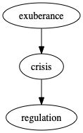
starting with a brief history of financial disaster, and ending with the current crisis in AI. But what crisis? We don’t have government bailouts of failed AI companies, or massive unemployment because of AI gone wrong as with financial crises.

The crisis facing us with AI is not so much a financial one as a societal one, as Cathy O’Neil persuasively argues, with thousands of decisions being made by algorithms in high-risk areas like educational opportunity and access to finance. When these go wrong, individuals suffer without the high profile boom of a financial crisis that makes it clear to everyone that something is amiss.

So regulators should step in and shut down high-risk AI, right? Note the name of the field is risk management and not risk elimination. As Bernadette Walter–the director of the quantitative risk modeling division of Deutsche Bank in my first post-academic job–stressed to her department, the job of risk management is to balance risk and return.

The EU’s proposed AI Act sets out this balance, recognizing both the potential for societal good as well as for crisis:

By improving prediction, optimising operations and resource allocation, and personalising service delivery, the use of artificial intelligence can support socially and environmentally beneficial outcomes and provide key competitive advantages to companies and the European economy. Such action is especially needed in high-impact sectors, including climate change, environment and health, the public sector, finance, mobility, home affairs and agriculture. However, the same elements and techniques that power the socio-economic benefits of AI can also bring about new risks or negative consequences for individuals or the society.

Discrete Geometry for Risk and AI

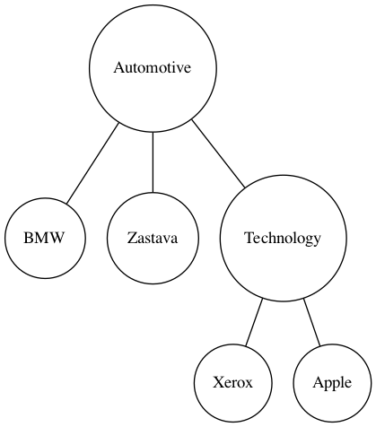
The second lecture introduced graphical models, probability polytopes and the geometry of Simpson’s paradox.

Graphical models occupy an interesting place in this history of AI, forming a sort of bookends separating the rules-based, expert system approaches up through the 80s, and more recently the dissatisfaction with deep learning as “curve fitting.” A key computer scientist for both of these bookends is Judea Pearl.

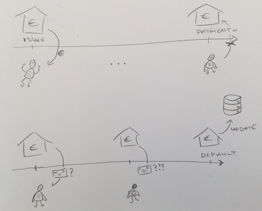
Though the focus was on directed graphical models, aka Bayesian Networks, I have a slide on undirected graphical models dedicated to my still favorite paper, Graphical Models for Correlated Default, by Bernd Sturmfels, I.O. Filiz, X. Guo and J. Morton.

The lecture material on probability polytopes also borrowed heavily from work and of Bernd Sturfmels along with his co-authors Seth Sullivant and Mathias Drton of Lectures Algebraic Statistics. It’s a lesson I learned during my PhD research, how good notation can convert a problem area and its solution space from opaque and complicated to transparent and straightforward.

Good notation for discrete probability spaces meant that my goal of generating interesting fake data subject to expectation constraints in the python package fake-data-for-learning a matter of applying the fundamental theorem of polytopes.

Of the three topics in this lecture, Simpson’s paradox is both the most accessible and the most surprising. It refers to a statistical phenomenon in which a trend exists for a population (e.g. splitting results of a clinical trial into treated and untreated populations) that then disappears or even reverses in subpopulations (e.g. further splitting the treated and untreated populations according to gender).

You may be wondering how machine learning algorithms deal with the strange statistics of Simpson’s Paradox–and you should–but that’s the topic of the final lecture .

The same useful notation from probability polytopes turned getting a geometric characterization of Simpson’s into a mess of scribbles over many pages in my notebooks into a system of a few quadratic equations or inequalities.

Correlation and Causality

In my first courses on statistics and early work in data science, I was warned that correlation and causation aren’t the same thing, but thereafter only heard about correlation-based methods. As with many things, correlation–and its fancier machine learning cousins–is so used because it 1.) is easy to calculate, and 2.) seems objective.

The third lecture starts with exploring what can go wrong when blindly accepting the correlation proxy (80% correlation annual deaths by venomous spiders and winning spelling bee word lengths anyone?) plus a brief history of causality from Aristotle to Judea Pearl.

Thanks to work by Judea Pearl and others, we can do more than complain about the inadequacies of correlation and curve-fitting. Using Pearl’s do calculus, this lecture showed how a causal analysis of a problem in insurance–estimating the impact of time-to-quote on customer’s acceptance or rejection of the quote–yields very different return-on-investment outlook when estimated causally compared to the more typical correlation-based estimate.

Risk and AI in Practice: Credit Scoring

The final lecture brought nearly everything from the first three together to tackle the problem of credit scoring. Based on historical data, how do we predict which customers should get a loan, and which should be rejected?

Access to finance is one of the high-risk AI applications singled out not only in the AI Act, but also the EU’s General Data Protection Regulation (GDPR). AI-based credit scoring has potential to increase access to the under-financed over status quo methods, but it also can–and apparently has–perpetuated past inequalities.

To give a simple example that both showed how to do data science properly and what can go wrong when you don’t, I generated artificial credit scoring data that incorporated two of the pathologies from the previous lectures: Simpson’s paradox and a collider, and then created around the data set a basic CI / CD machine learning pipeline.

The embedded Simpson’s paradox in the dataset meant that female populations overall seemed a worse credit risk, but in each of the occupation sub-populations the female default rate was better than the male counterpart. But this wasn’t enough by itself to trick the three machine learning algorithms we considered into rating women worse (with more complicated datasets relying more on regularized algorithms, you’d maybe see the algorithms getting tricked by Simpson’s paradox).

So I added an extra feature of account-activity that–in the data generating process–was a collider resulting in a high and spurious correlation between gender and default. You may think this is a cheat to put in a field with the causal direction going from target (default) to a field (account-activity), but I have come across examples of business and data collection practices that–if missed by data scientists–can product such data leakage.

Maybe it wouldn’t have made a difference to the students, but alongside a more traditional Jupyter notebook implementation of the model selection and training process, I implemented a basic but tested pipeline. I was curious about Data Version Control, and still like some features of it, but ended up focusing on a combination of old-school Git + a bash script with test coverage.

We wrapped up on a definite positive note: machines won’t replace the bright, dedicated minds in the lecture hall any time soon. I won’t make a prediction here in print, but I don’t see AI in the near future meeting the demands facing the masters students in their first job, namely to

• to think deeply about the data and process you feed into your AI algorithm,
• to think deeply about modular code design with test coverage, and
• to think deeply about the impact of your work on society.

Takeaways

The next generation

The masters students showed not only the curiosity and appetite for learning you might expect from top students, but also an interest in using their expertise and creativity for the good of society. This gives me hope.

Rigorous practice rather than Luddism for human-centered AI

Sure, there will be applications of AI for which a Luddite “Don’t go there” is the appropriate response, but for the examples of the workshop, rigorous practice is what ensures your AI model is compatible with the values articulated in the EU’s AI Act.

Modern software practices like MLOps (aka CI/CD for ML) are effective tools for managing operational risk

A big change for this year’s workshop was to think of the workshop repository like an application, and automate everything that made sense to automate. I already had unit tests for code I had written, but I was still manually checking that notebooks actually ran without error, and manually compiling and versioning the (laTeX) slides, all manual processes that could and did result in error and last-minute frantic fixes.

So what is the critical functionality of the workshop repository that should be tested and delivered like other software?

1. Continuous integration: All example and exercise notebooks should run without error on the students’ laptops, including a machine learning pipeline for credit scoring.

2. Continuous delivery: All slides should be generated based on the tested code state on the main branch.

Was my extra effort worth it? Yes. Did I eliminate all errors for the workshop? Not all, but I reaped the expected benefits, namely

Preservation of my own sanity at crunch time

For the typos and other bugs that popped up while preparing and even during the workshop, I could focus on the task at hand, and not the (now-automated) manual steps of re-running laTeX builds and manually adding them to version control.

The biggest case of sanity-preservation via automation was in coming up with synthetic data for credit scoring that exhibited desired characteristics. In addition to data versioning, I wrote a ratchet test to automatically test the generated data and fitted models had the desired traits.

Improved mean-time-to-recovery

I didn’t keep precise statistics, but my gut says we had the same percentage of dependency install mishaps on student laptops this year as last, but (again, gut-based) the process of diagnosing and fixing issues went faster.

One benefit of the CI / CD pipeline–which tested custom code and notebook execution on Windows, Mac and Linux operating systems–was that I could focus faster on what was really wrong. Specifically, I knew it wasn’t just a Windows thing, my go-to explanation in the last round.

In general, this faster-focus-on-root-cause benefit is one of the reasons I still practice and adore test-driven-development.